Tables
This section explains how to create and format think-cell tables in PowerPoint. By default, tables consist of grouped text boxes that resize automatically based on their contents. To learn more about text boxes, see Text boxes. Table cells can also consist of Harvey balls, checkboxes, and other elements.
For general instructions on formatting and arranging tables and other think-cell elements, see Shapes and elements.
Insert tables
To insert a table onto your slide, on the PowerPoint ribbon, select Insert > think-cell > Elements > Table ![]() .
.
In think-cell Suite, you can create tables directly from Excel, update tables with external data, and match table formatting to Excel. To learn more, see Create tables from Excel.
Create tables from individual elements
You can create a table using any combination of Text boxes, Harvey balls and checkboxes, Rounded rectangles, Pentagons and chevrons, and Images and icons.
To create a table from any of these elements, follow these steps:
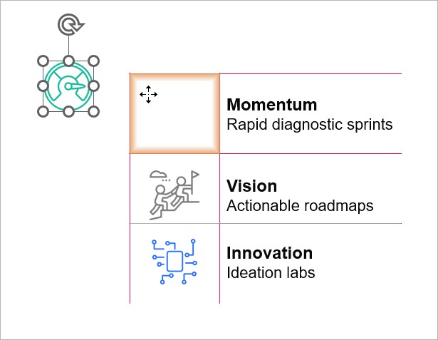
- On your slide, insert the elements that you want to include in your table. For example, insert some icons and text boxes.
- Arrange the elements in a tabular layout.
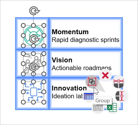
- Select the elements. Right-click the selection to open the context menu, then select Group
 .
.
To change the content type of a table cell—for example, to change a text box into a Harvey ball—see Choose cell content type.
In think-cell Suite, you can Create tables with datasheets from individual elements.
Add or delete table rows and columns
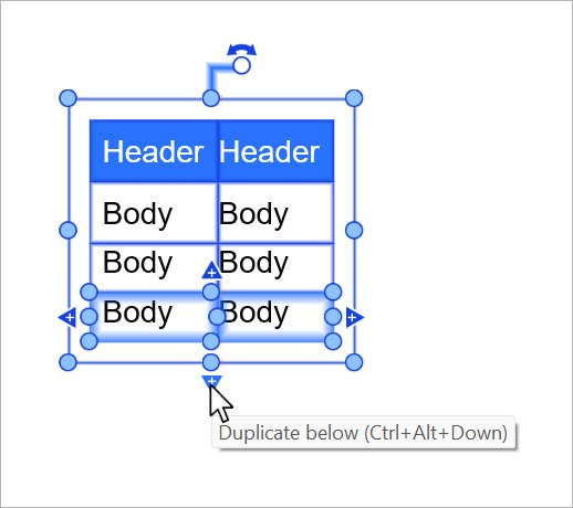
To add rows or columns to a table, follow these steps:
- Select a row or column (see Select objects). Arrows appear on each side of your selection.
- Select the arrow on the side where you want to add the new row or column. Alternatively, select and hold Ctrl+Alt, then use the arrow keys to create rows or columns.
To delete table rows or columns, select the row or column, then select Del or Backspace. Alternatively, right-click the selection to open the context menu, then select Delete

Resize tables
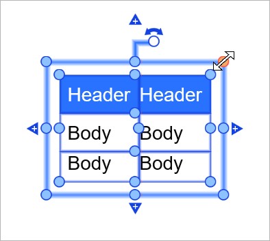
To resize a table, follow these steps:
- Select the table.
- Drag one of the resize handles on the table's outer selection frame.
Automatically resize table rows and columns to fit their contents
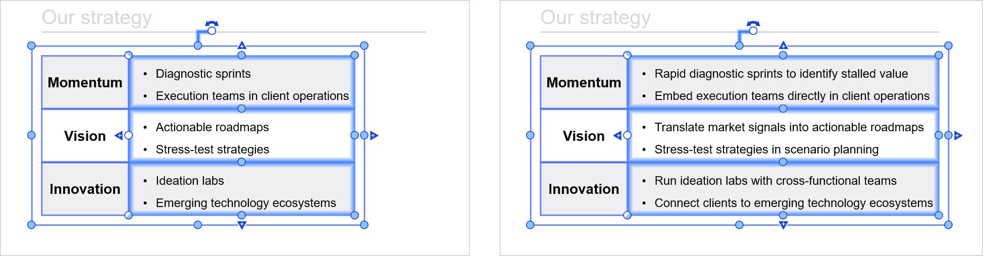
Table rows and columns can automatically resize to fit their contents. You can turn automatic resizing on and off, and chose the direction in which a row or column grows or shrinks, by unlocking and locking the edges of a row or column.
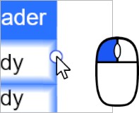
An unlocked edge can automatically move to fit the row's or column's contents. An unlocked edge has a blue resize handle 
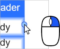
A locked edge doesn't move, even when the contents of the row or column change. A locked edge has a white resize handle 
Groups of elements, including tables, have an additional outer selection frame. The edges of a table and its outer selection frame always share the same locked or unlocked state. To lock or unlock the outer edges of a table, you can click or right-click the resize handles of the inner or outer selection frame.
To learn more, see Lock and unlock elements.
Automatic resizing examples
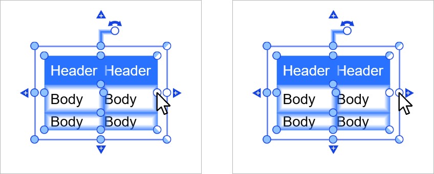
To automatically fit the height of a row to its contents so that the top edge stays locked and the bottom grows or shrinks, lock the top edge and unlock the bottom edge.
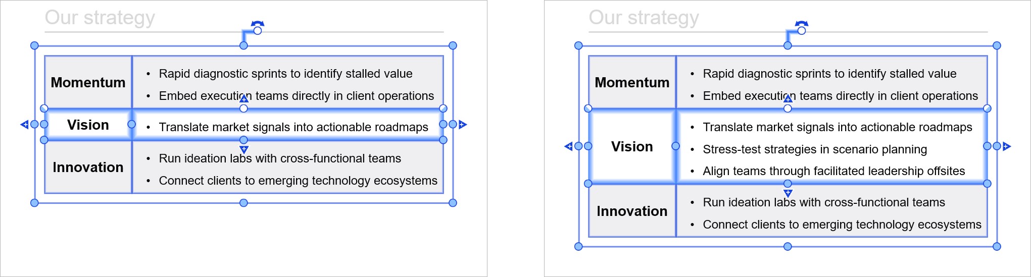
To automatically fit the width of a column to its contents so that the left edge stays locked and the right side grows or shrinks, lock the left edge and unlock the right edge.
To turn off automatic resizing of a row's height, lock its top and bottom edges.
To turn off automatic resizing of a column's width, lock its left and right edges.
Dynamically align tables with other elements
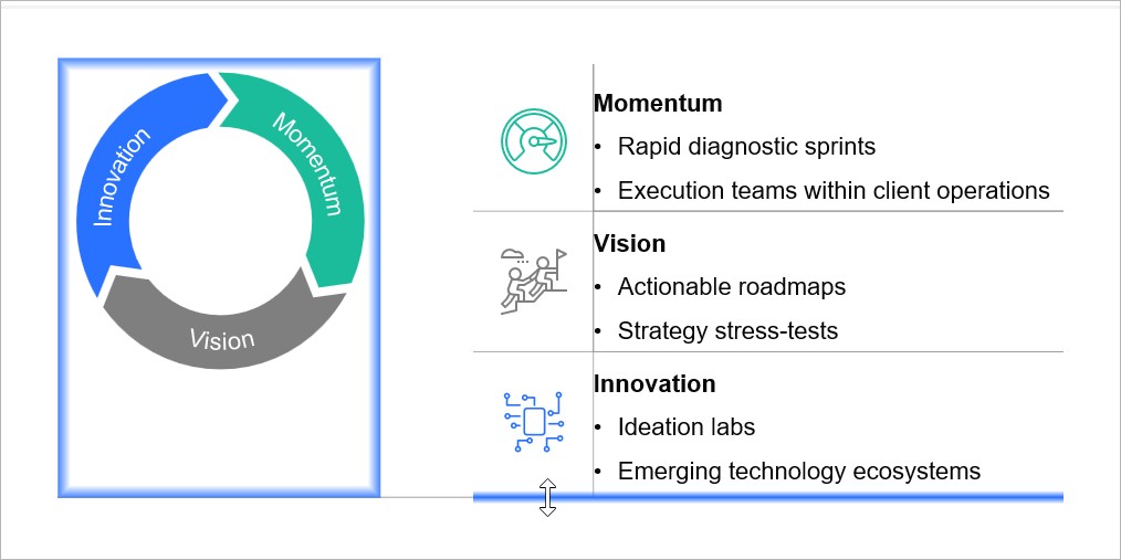
You can create dynamic alignments between tables and other think-cell elements. When you edit the table, the other elements move or resize to preserve the alignment.
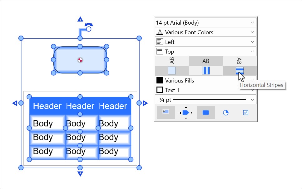
For example, you can align a table and an image so that the image always matches the height of the table, even when you edit the table's contents.
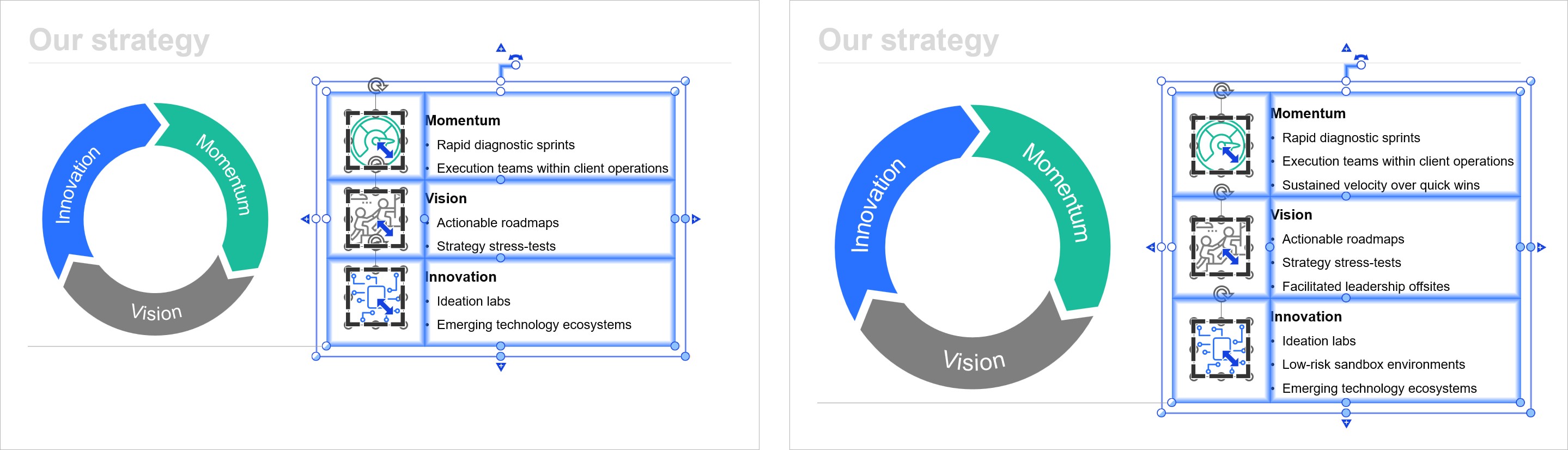
In this example, the bottom edges of the image and the table are dynamically aligned, as indicated by a thin gray line between the edges. Once you move one of the elements or certain edges, the dynamic alignment breaks (see Break dynamic alignments).
To create a dynamic alignment between a table and another element, follow these steps:
- Before you dynamically align the edges that you want—in this example, the bottom edges of the image and table—you may want to lock some of the elements' other edges so that they don't move when you edit the table. A locked edge has a white resize handle
In this example, the following edges are locked:- The top edges of the image and table, to preserve their alignment.
- The right edge of the image and left edge of the table, to preserve the space between them.
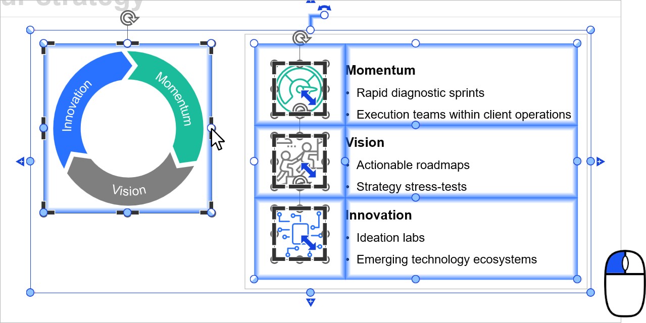
- Select one of the elements that you want to include in your dynamic alignment—for example, the image.
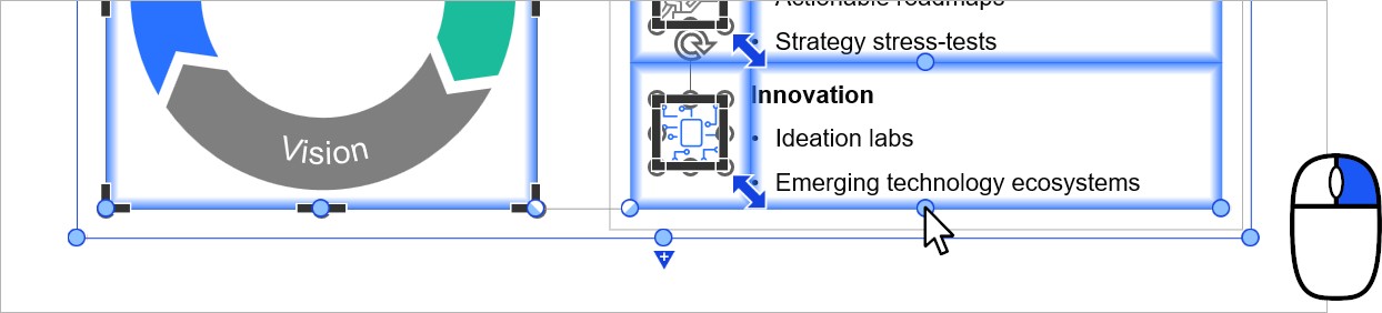
- Start dragging the resize handle of the edge that you want to align—in this example, the handle of the bottom edge.
- While dragging the resize handle, move the mouse pointer onto the edge of the other element that you want to align to. The edge that you're aligning to is highlighted in blue, and a thin line appears between the edges. Release the mouse button.
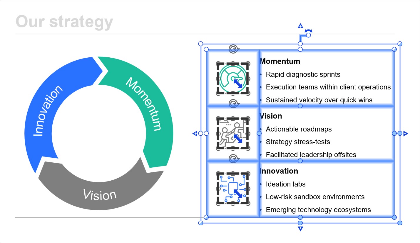
- Make sure that the edges that you want to dynamically align are unlocked—for example, the bottom edges of the image and table. An unlocked edge has a blue resize handle
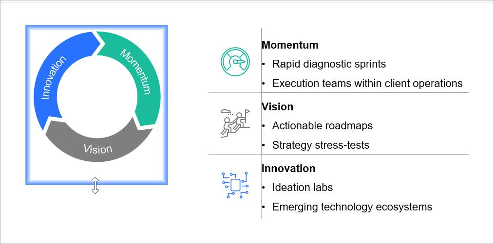
When you edit the table, the dynamic alignment will persist. In this example, the image resizes so that the bottom edge of the image is always aligned to the bottom edge of the table.
Break dynamic alignments
The following actions will break a dynamic alignment by locking one or more edges:
- Move one of the dynamically aligned elements.
- Left-click the resize handle of a dynamically aligned edge.
- Drag the resize handle of a dynamically aligned edge.
- Drag the resize handle of an edge that's opposite a dynamically aligned edge. For example, if the right edge is dynamically aligned, moving the left edge will break the alignment.
Format tables
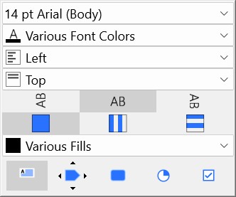
To format a table, select the table to open the mini toolbar. By default, the mini toolbar has the following formatting options:
- Font and font size (see Change the font and font size)
- Font color (see Change the font color)
- Horizontal and vertical alignment (see Change the text alignment)
- Text direction (see Change the text direction)
- Vertical and horizontal stripes (see Apply alternating fills to rows or columns)
- Fill (see Fills)
- Cell content (see Choose cell content type)
You can select and format individual cells, columns, rows, or the entire table (see Select objects).
Depending on the cell content, other formatting options appear on the mini toolbar. For example, if a table cell contains a checkbox, the mini toolbar displays checkbox formatting options (see Checkboxes).
You can apply PowerPoint's built-in paragraph formatting options to text in tables. To learn more, see Apply PowerPoint text formatting.
Apply alternating fills to rows or columns
You can make your tables easier to scan by applying alternating fills to table rows or columns. To apply alternating fills, follow these steps:
- Select the table or the cells that you want to apply alternating fills to.
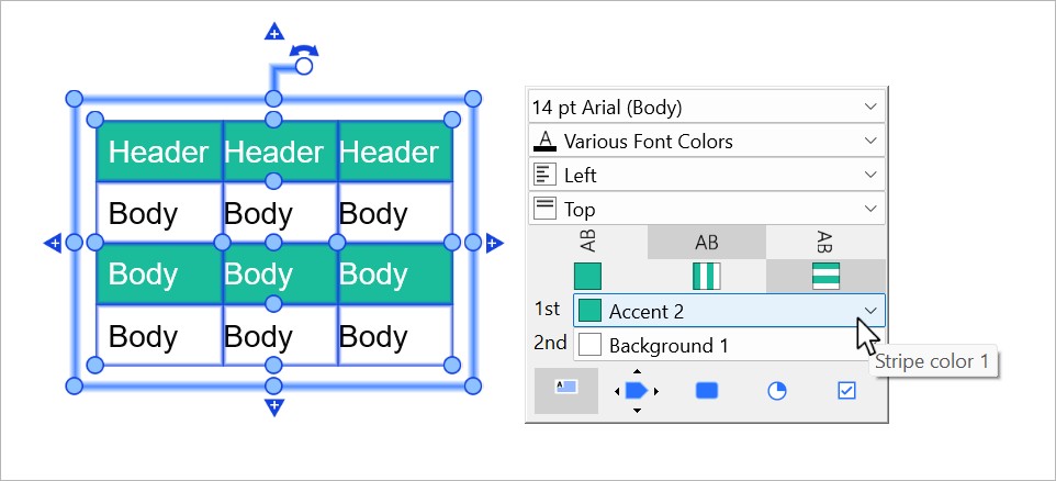
- On the mini toolbar, select Vertical Stripes


After you apply alternating fills, on the mini toolbar, the Stripe color 1 and Stripe color 2 menus replace the Fill menu. By default, think-cell uses no fill for Stripe color 1 and the Accent 1 color of your PowerPoint theme as Stripe color 2. To change the alternating fills, on the Stripe color 1 and Stripe color 2 menus, select the fills that you want.
To use another element's fill as Stripe color 1, select the element as the reference object (see Select a reference object).
To remove alternating fills, select the table or the cells to open the mini toolbar, then select No Striping 
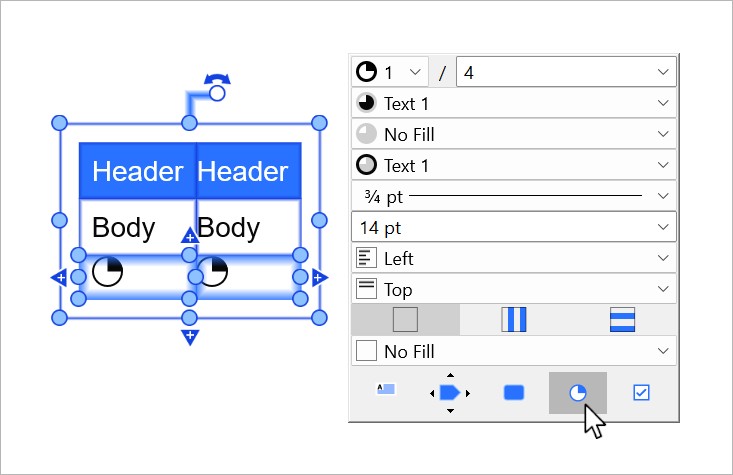
Choose cell content type
Instead of text boxes, table cells can consist of other elements. To change a table cell's content type, select the cell to open its mini toolbar, then choose one of the following options:
- Text Box
 (see Text boxes)
 - Pentagon/Chevron
 (see Create process flows)
 - Rounded Rectangle
 (see Rounded rectangles)
 - Harvey Ball
 (see Harvey balls)
 - Checkbox
 (see Checkboxes)
Need to troubleshoot?
Check our knowledge base