Excel data links
- Home
- Resources
- User manual
- think-cell Charts: Data visualization
- External data links
- Excel data links
Use Excel data in your presentation by linking existing elements to Excel or creating new elements directly from Excel. When the data in Excel changes, linked elements stay up-to-date without the need to manually copy and paste values from Excel.
This page explains how to create data links between Excel and PowerPoint, and how to manage linked Excel ranges and adjust them to fit your presentation's needs. To learn how to manage linked elements and update their data, see Manage the data in linked elements.

Link elements in your presentation to Excel
Use Excel data in think-cell elements and presentation text on your slides. When you link an element to an Excel range, the data in the linked cells replaces the corresponding data in the element.
You can Format and style elements that you link to Excel like any other think-cell element, or Match element formatting to the linked data range to control the look of your linked elements from Excel.
Link charts and other elements to Excel
Use Excel data in think-cell charts, tables, Harvey balls, and checkboxes in your presentation. To do so, follow these steps:
- In Excel, select the cells that contain the data that you want to use in the element.
- On the ribbon, select Insert > think-cell > Link To PowerPoint > To Existing Element

- In PowerPoint, select the element.
Alternatively, follow these steps:
- In Excel, select the cells that contain the data that you want to use in the element.
- In PowerPoint, do one of the following:
- Select the element, then, on the ribbon, select Insert > think-cell Data > New Excel Link.
- Right-click the element to open its context menu, then select Establish Excel Link
 .
.
If the data layouts of Excel ranges and charts and tables in your presentation don't match, you can Adjust linked ranges to match element data layouts without editing individual cells.
Link presentation text to Excel
Link text in a think-cell or PowerPoint object to Excel and use the linked Excel data to replace or supplement the text. You can link text in any object in your presentation to Excel, except for PowerPoint tables and SmartArt graphics.
To link presentation text to Excel, follow these steps:
- In Excel, select the cell that contains the data that you want to use in the object.
- In PowerPoint, choose how you want to use the linked Excel data:
- To replace the text in the object with the Excel data, select the object.
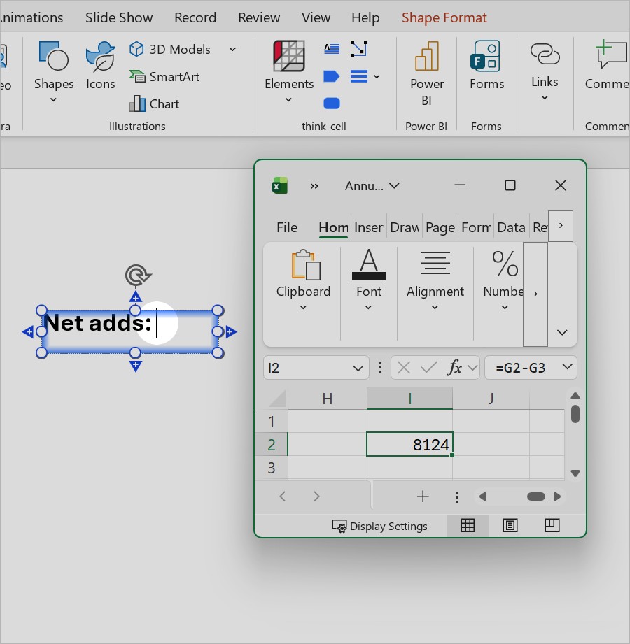
- To replace a part of the text in the object with the Excel data, select the text that you want to replace.
- To add the Excel data without replacing the text in the object, place the cursor where you want the Excel data to appear.
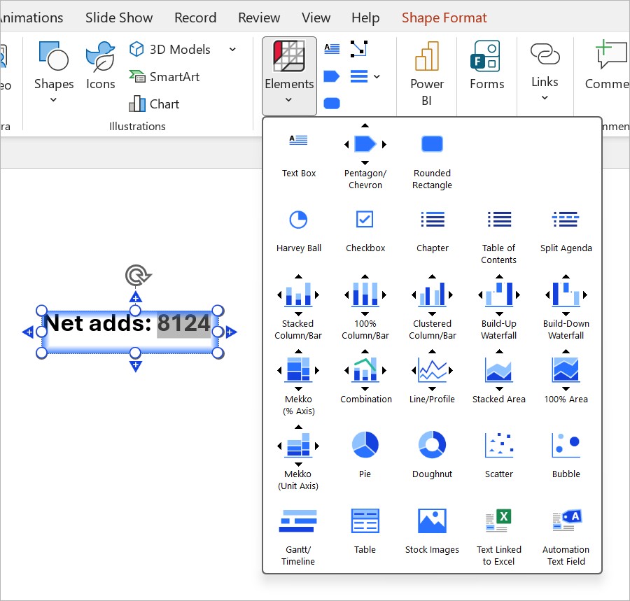
- In PowerPoint, on the ribbon, select Insert > think-cell > Elements > Text Linked to Excel

Create new elements from Excel
When you want to use Excel data as the starting point for new elements, you don't have to create the elements in PowerPoint and link them to Excel afterwards. You can create linked charts, tables, Harvey balls, checkboxes, and images in your presentation directly from Excel.
You can Format and style elements that you create from Excel like any other think-cell element, or Match element formatting to the linked data range to control the look of your linked elements from Excel.
Create charts from Excel
To create a chart from Excel, follow these steps:
- In Excel, select the cell range that you want to use in your presentation.
- On the Excel ribbon, select Insert > think-cell > Link To PowerPoint, then select the chart type that you want. PowerPoint opens.
- In PowerPoint, place the chart on a slide.
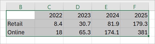
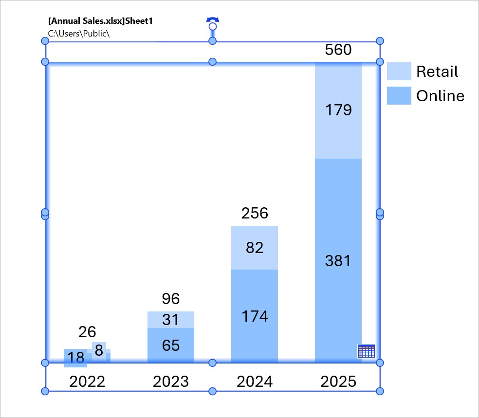
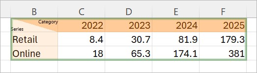
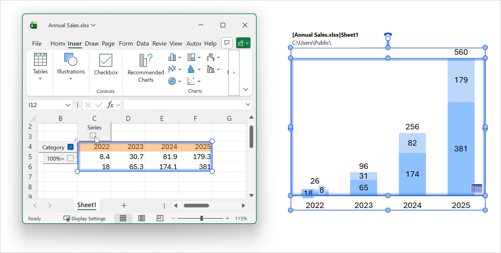
The Excel range in the following example matches the default layout for a stacked column chart: rows are series and columns are categories.
If the data layout of a chart and its linked range doesn't match, Adjust linked ranges to fit the chart data layout without editing individual cells.
Create tables from Excel
There are three ways to recreate your Excel tables as think-cell elements in PowerPoint:
To update tables or adjust their update settings, see Manage the data in linked elements and Manage linked data with the Data Links dialog. You can Format tables that you create from Excel—except for images of tables—like any other think-cell table.
Create tables
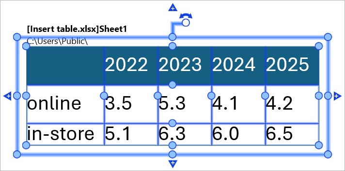
To create a think-cell table from Excel, follow these steps:
- In Excel, select the cell range that you want to include in the table.
- On the Insert tab, in the think-cell group, select Link to PowerPoint > Table. PowerPoint opens.
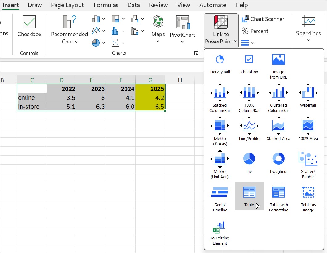
- In PowerPoint, place your table on a slide.
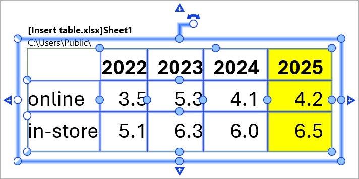
Create tables with Excel formatting
Create a table in which most formatting options—such as font style, fill color, and text alignment—initially match those specified in your Excel sheet. For more information, see Match element formatting to the linked data range.
To create a table with Excel formatting in your presentation, follow these steps:
- In Excel, select the cell range that you want to include in the table.
- On the Insert tab, in the think-cell group, select Link to PowerPoint > Table with Formatting. PowerPoint opens.
- In PowerPoint, place your table on a slide.
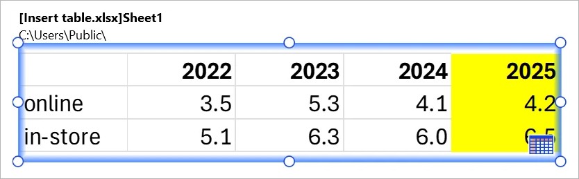
Create images of tables
Create an image of a table that matches your Excel sheet. Update the image from Excel like any other linked element (see Manage the data in linked elements). In PowerPoint, images of tables behave like any other image. You can only edit the contents and formatting of an image of a table using its linked Excel sheet. To insert a table from Excel that you can edit and format in PowerPoint, see Create tables and Create tables with Excel formatting.
To create an image of a table in your presentation, follow these steps:
- In Excel, select the cell range that you want to include in the table.
- On the Insert tab, in the think-cell group, select Link to PowerPoint > Table as Image. PowerPoint opens.
- In PowerPoint, place your table on a slide.
Create Harvey balls and checkboxes from Excel
Create and control the status of Harvey balls and checkboxes directly from an Excel workbook. To learn more about Harvey balls and checkboxes, see Harvey balls and checkboxes.
Create Harvey balls from Excel
To create a Harvey ball from Excel, follow these steps:
- In Excel, in an empty cell, specify the number of filled Harvey ball segments by entering one of the following:
- An absolute number between
0and4, which is the maximum number of Harvey ball segments by default - A percentage between
0%and100% - A formula that results in either an absolute number between
0and4or a percentage between0%and100%
- An absolute number between
- Select the cell, then select Insert > think-cell > Link to PowerPoint > Harvey Ball

- In PowerPoint, place the Harvey ball on a slide.
You can Change the number of segments in a Harvey ball that you created from Excel like any other Harvey ball. To change the completion state of a Harvey ball from Excel, in the linked cell, enter another value or formula. To learn more about updating linked elements, see Manage the data in linked elements.
Create checkboxes from Excel
To create a checkbox from Excel, follow these steps:
- In an empty cell, enter a checkbox symbol shortcut or a formula that results in a shortcut:
- Empty checkbox (☐):
0or an empty space - Check symbol (✓):
1orv - X symbol (✗):
2orx - Custom checkbox symbol: the symbol shortcut that you specified in your think-cell style file (see Customize the default checkbox styles).
- Empty checkbox (☐):
- Select the cell, then select Insert > think-cell > Link to PowerPoint > Checkbox

- In PowerPoint, place the checkbox on a slide.
To change the checkbox symbol from Excel, in the linked cell, enter another checkbox symbol shortcut or formula. To learn more about updating linked elements, see Manage the data in linked elements.
Create images from Excel
Insert an image into your presentation from an Excel cell that contains the image's URL or local file path. To do so, follow these steps:
- In Excel, in an empty cell, enter the image's URL. If the image is stored on your device, enter the file path to the image, starting with
file://.
- Select the cell that contains the URL or file path.
- On the Excel ribbon, select Insert > think-cell > Link to PowerPoint > Image from URL. PowerPoint opens.
- In PowerPoint, place the image on a slide.

You can also replace an image on your slide with an image from a URL or file path in Excel. To do so, follow these steps:
- In PowerPoint, select the image that you want to replace.
- In Excel, select the cell that contains the URL or file path of the image that you want to use.
- Choose from the following options:
- In Excel, on the ribbon, select Insert > think-cell > Link To PowerPoint > To Existing Element
- In PowerPoint, on the ribbon, select Insert > think-cell Data > New Excel Link. Alternatively, right-click the image to open its context menu, then select Establish Excel Link .
- In Excel, on the ribbon, select Insert > think-cell > Link To PowerPoint > To Existing Element
Switch between linked images using Excel formulas
Switch between different images on your slide from Excel using formulas and cell references that result in image URLs or file paths. To do so, follow these steps:
- In Excel, create a formula that results in the image URLs or file paths that you want to use.
- Select the cell that contains the formula.
- On the Excel ribbon, select Insert > think-cell > Link to PowerPoint > Image from URL. PowerPoint opens.
- In PowerPoint, place the image on a slide.
- To switch images, change the value that the formula uses, then update the linked image in PowerPoint.
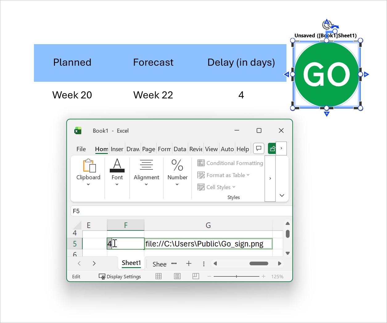
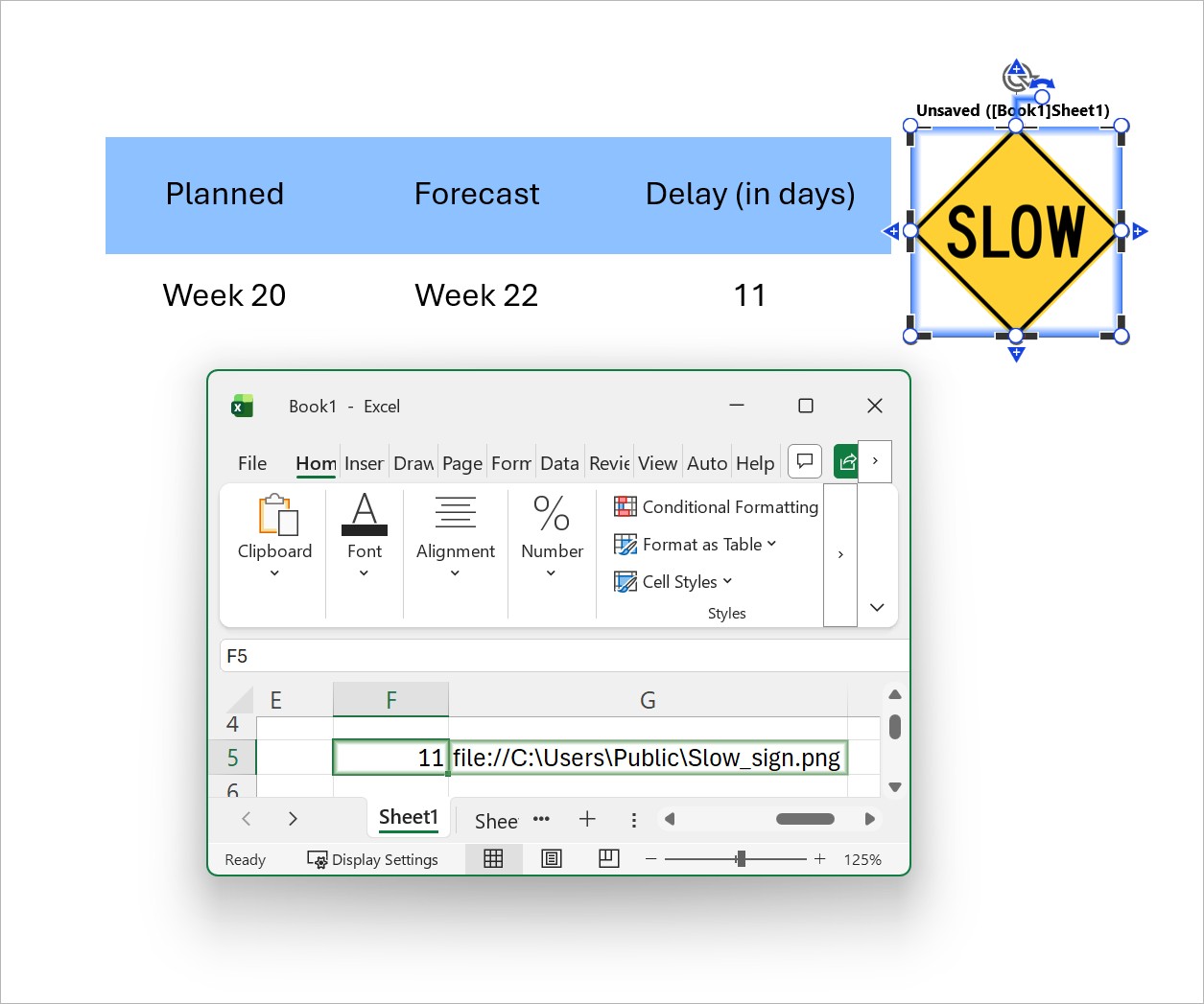
For example, the following Excel formula returns one of two image file paths, depending on the value in cell F5:
=IF(F5<10,"file://C:\Users\Public\Go_sign.png","file://C:\Users\Public\Slow_sign.png")When you insert or replace an image on your slide with a data link to the formula cell, the linked image changes depending on the value in cell F5:
Manage linked Excel ranges
Linked Excel ranges have color-coded data link frames.
The color of a data link frame indicates the linked range's status.
|
Frame |
Data link status |
|---|---|
|
|
There are open presentations with linked elements that use the data in the linked range. |
|
|
No open presentation contains linked elements that use the Excel range. Possible reasons are:
|
|
|
The data link frame is selected. |
When linked Excel ranges don't match the needs of your presentation perfectly, you don't have to move cells around or edit their contents. You can Adjust linked ranges to match the data layouts of linked elements, or Arrange Excel data to fit linked elements to organize it for linked elements.
You don't need to have PowerPoint open while adjusting linked ranges or compiling data. To see the changes in PowerPoint, open a presentation with linked elements that use the data in the linked range and update the linked elements (see Manage the data in linked elements).
Adjust linked ranges
There are three different ways you can adjust linked Excel ranges after you link them to elements in PowerPoint:
- Move the data link frame
- Add or remove rows and columns
- Transpose and edit the data layout of linked ranges
Move the data link frame
Include different cells in a linked range by moving the data link frame. To do so, follow these steps:
- Select the data link frame around the linked range.
- Drag and reposition the data link frame over the cells that you want to include in the data link.
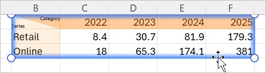
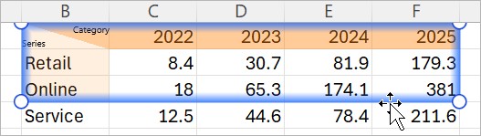
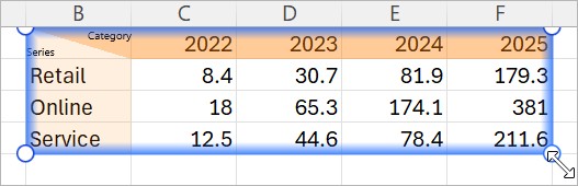
Add or remove rows and columns
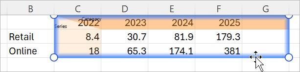
When you need to add another series to a linked chart or remove a row from a linked table, resize the data link frame to include or exclude cells. To do so, follow these steps:
- Select the data link frame around the linked range.
- Resize the data link frame by selecting and dragging a corner handle.
Transpose and edit the data layout of linked ranges
Linked elements in PowerPoint use default data layouts to interpret and display Excel data. For example, when you create a column chart from an Excel range, the chart uses rows as series and columns as categories by default (see Create charts from Excel).
You can change how linked elements interpret and display Excel data without editing or moving the data. To do so, transpose or edit the data layout of linked ranges.
Transpose linked ranges
To switch between rows and columns of linked cells to represent certain values in linked elements, such as category and series labels, you can transpose linked Excel ranges. Transposing a linked range doesn't change or move the data in Excel; it only changes how the linked elements display the data.
To transpose a linked range, right-click the data link frame around the linked range, then select Transpose Link 
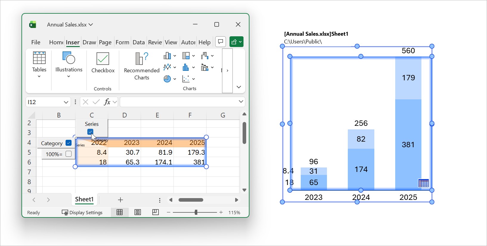
Edit the data layout of linked ranges
Specify whether certain rows and columns in linked Excel ranges represent data values or optional information in linked elements, such as series and categories, or a 100%= row (see Absolute and relative values). To do so, follow these steps:
- In Excel, right-click the data link frame around the linked range, then select Edit Data Layout

- Use the checkboxes to specify how think-cell interprets the rows and columns in the linked range.
Arrange Excel data to fit linked elements
When you link elements to Excel, the data that you want to use may be mixed with data that you don’t need, or it may be arranged in a format that you don’t want to change. If you need more flexibility when fitting linked Excel data to your presentation, consider the following options:
- Fill empty cells on the worksheet with cell references that mirror the values in other cells, then link the cells that contain references to your presentation. For example, enter
=B5in cell F8 so that F8 always shows the value in cell B5. To use the data in cell B5 without affecting the cell, link cell F8 to your presentation. - Use Excel cell references across worksheets, and collect all data that you want to use on a dedicated interface sheet. Interface sheets allow you to adapt linked data to your presentation without altering the original worksheets that contain the data. For example, you can consistently round the values that will appear in linked charts by using think-cell round on the interface sheet cells (see Excel data rounding).
- To exclude cells in a linked range from a chart, use Excel's Hide or Group and Outline function. To show hidden data in the chart again, select Unhide in Excel, then update the chart.
View duplicate linked ranges
When you create a data link between PowerPoint and Excel, think-cell assigns a data link ID to the linked Excel range. If you create a copy of a workbook or worksheet that contains a linked range, the linked ranges in the original and the copy share the same data link ID.
When there are multiple open linked ranges with the same data link ID, think-cell recognizes them as duplicates, and color-coded tabs appear under each linked range that show all open duplicates. Tab colors indicate the status of linked ranges.
|
Tab |
Data link status |
|---|---|
|
|
There are open presentations with linked elements that use the data in the linked range. |
|
|
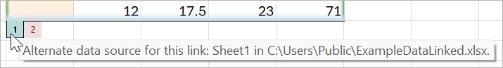
The linked range is an unused alternate data source (see Switch to alternate data sources). |
When you hover over a tab, a tooltip shows the worksheet name and workbook file path that contains the linked range.
To open a worksheet that contains a specific linked range, select its tab. Selecting the tabs in Excel doesn't change the data source of linked elements in PowerPoint. To change the data source of linked elements, Switch to alternate data sources with the Data Links dialog.
Need to troubleshoot?
Read our knowledge base