KB0188: How can I create a linear trendline in a line chart?
- Home
- Resources
- Knowledge base
- KB0188
To create a trendline in a line chart, add a new series to the line chart, then calculate its values to form a trendline, e.g., by using the TREND function of Excel:
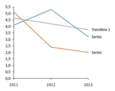
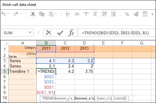
- Open the internal datasheet and add a new series, e.g., "Trendline 1".
-
Calculate the first value of the trendline using the TREND function:
- type "
=TREND(" or use the Insert Function (fx) menu in Excel. - Select all "known y" values and press F4 (e.g., "$B$3:$D$3").
Enter Excel's arguments separator, e.g., "," (comma).
(Note that the character expected by Excel as an arguments separator depends on your Windows regional settings. To see the correct character for your region refer to the Excel tooltip appearing while you enter the formula). - Select all "known x" values and press F4 (e.g., "$B$1:$D$1").
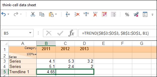
Enter Excel's arguments separator. - Select the first x value (e.g., "B1") and press ENTER.
Note: By pressing F4 the cell reference type of the selected cells will change to absolute cell references. This way the selection will stay exactly the same when this formula is copied and will not be adjusted according to the new position.
- type "
-
Select the first value of the new trendline and copy the function by using Excel's Auto Fill feature, dragging the fill handle in the cell's lower right corner to the right until the cell of the last value is selected as well.
Note: If you receive a #VALUE! error, check if the "known x" and/or "known y" values were auto-filled incorrectly - you may have used relative references when setting up the formula. In this case change the cell reference type of the "known x" and "known y" values as described in step 2, using F4. Repeat step 3 afterwards.