7. Column, line and area chart

Contents
- 7.1
- Column chart and stacked column chart
- 7.2
- Clustered chart
- 7.3
- 100% chart
- 7.4
- Line chart
- 7.5
- Error bars
- 7.6
- Area and area 100% chart
- 7.7
- Combination chart
7.1 Column chart and stacked column chart
|
Icon in Elements menu: |
|


In think-cell, we do not distinguish between simple column charts and stacked column charts. If you want to create a simple column chart, enter only one series (row) of data in the datasheet. For a quick tour of the column chart, refer to the example in the chapter 4. Introduction to charting.
Bar charts in think-cell are simply rotated column charts, and can be used exactly as column charts. In addition, you can create butterfly charts by placing two bar charts “back-to-back”. To do so, apply the functions rotation (see 3.3 Rotating and flipping elements) and same scale (see 8.1.4 Same scale). Then remove the category labels for one of the charts.

For the steps to create a stacked clustered chart, see 7.2 Clustered chart.
To change the column width, select a segment and drag one of the handles at half the height of the column.

The tooltip shows the resulting gap width while dragging. A larger column width results in a smaller gap width and vice versa, as the chart width is not altered when column widths are changed. The gap width is displayed as a percentage of the column width, i.e., a value of 50% means that each gap is half as wide as a column.
Changing the column width for one column will change it for all other columns as well. All columns always have the same width. For a chart with variable column widths depending on your data, see 10. Mekko chart. To make individual gaps wider, see 8.1.7 Category gap.
7.2 Clustered chart
|
Icon in Elements menu: |
|


The clustered chart is a variant of the stacked column chart, with the segments arranged side-by-side.
A clustered chart can be combined with a line chart by selecting a segment of a series and choosing Line from the chart type control of this series.
If you want to arrange stacks of segments side by side, you can create a stacked clustered chart.

To create a stacked clustered chart, follow these steps:
- Insert a stacked chart.
- Select a segment and drag the column width handle at half the height of the column until the tooltip shows 0% gap.
- Click onto the baseline where you want to insert a category gap and drag the arrow to the right until the tooltip shows 1 Category Gap; this has to be repeated for all clusters.
If there is an even number of stacks in a cluster, the label cannot be centered to the whole cluster. Use a PowerPoint text box as a label in this case.
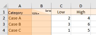
7.3 100% chart
|
Icon in Elements menu: |
|

The 100% chart is a variation of a stacked column chart with all columns typically adding up to the same height (i.e., 100%). The labels of the 100% chart support the label content property, which lets you choose if you want to display absolute values, percentages, or both (6.5.5 Label content).

With think-cell, you can create 100% charts with columns that do not necessarily add up to 100%. If a column totals to more or less than 100%, it is rendered accordingly. For details about filling in the datasheet refer to 5.2 Absolute and relative values.
7.4 Line chart
|
Icon in Elements menu: |
|


The line chart (also called a profile chart when rotated by 90°) uses lines to connect data points belonging to the same series. The appearance of the line chart is controlled by the line scheme, line style and marker shape controls in the floating toolbar. See 3.8 Formatting and styling for details on these controls. Labels for the data points are not shown by default but may be displayed using the line chart 
If the category values of a line chart are strictly increasing numbers or dates and can be interpreted as such according to the axis label number format, then the X-axis will automatically switch to a value axis (see 8.1.1 Value axis). When dates are used the date format can be changed by multi-selecting all category labels (see 3.5.1 Multi-selection) and typing a date format into the control (see 13.8 Date format codes). If you want to show more labels than would fit next to each other horizontally you can use label rotation (see 6.3.1 Label rotation).
The X-axis can only switch from category to value mode if the following conditions are met:
- All category cells in the datasheet contain numbers and Excel’s cell format is also set to General or Number or all category cells in the datasheet contain dates and Excel’s cell format is also set to Date.
- The numbers or dates in the category cells are strictly increasing from left to right.
-
The Y-axis is not set to Crosses Between Categories (see ). If only this requirement is preventing a switch to the value axis mode, you can use


If the X-axis has been deleted, the data is displayed as for a category axis.
The line chart can also display a second value Y-axis. Please refer to 8.1.6 Secondary Axis for further information.
If Use Datasheet Fill on Top is selected (see 3.8.2 Color scheme), the fill color from Excel’s cell formatting is used in the following way:
- The fill color of the cell containing the series name determines the line color.
- The fill color of each data point’s cell determines the marker color for this data point.
7.4.1 Smoothed lines
If you prefer a smoother appearance of the lines in a line chart, you can turn on this setting. First right-click on the desired line, then use the 
7.4.2 Interpolation
In line, area and area 100% charts, missing values are linearly interpolated by default. The 
In line charts, interpolation can be enabled and disabled for individual series in a chart. In area charts, it can only be applied to the whole chart, because the series stack on each other.
7.5 Error bars
Error bars can be used to indicate deviations in the line and stacked chart. By means of the error bars the following chart can be created.

- Create a line chart with three series. The first series reflects the upper deviation, the second series reflects the mean and the third series reflects the lower deviation.
- Right-click the center line and choose


Select one of the error bars to change the marker shape and color for the upper and lower deviation and the line type of the bar for all error bars. You can also select an individual error bar marker to change the properties for this marker only.
A handle appears at each end when you select an error bar. You can drag these handles to select which lines the error bars should span. You can also visualize intervals instead of the deviation around a central value if you set the error bar to only span two adjacent lines.
7.5.1 Football field chart
Using a rotated line chart and error bars, you can also create football field charts. They can be used to visualize the low and high values for an item and the spread between them.

To create a football field chart:
- Create a line chart rotated to the right (a profile chart)
- Enter the low and high values in the datasheet
- Select both the lines for low and high values
- Right-click and choose Add Error Bars from think-cell's context menu
- Select one error bar and format both the bar and data points for low and high values as desired. You would typically switch to a thick error bar, e.g., 6pt in football field charts.
- Right-click the chart background and select Add Gridlines from the context menu. To style all of them, select any one of them and press Ctrl+A to select all. You can then choose formatting options from the floating toolbar, such as a lighter color.

If your first data range is placed on top of the horizontal Y-axis, you can either modify the axis extent of the vertical axis (see 8.1.1 Value axis) or drag the Y-axis upwards. Note that in the latter case, the vertical axis will turn into a category axis, leading to data points being evenly spaced vertically instead of based on the numerical or date values in the category row.
Using more than two series and by adding multiple error bars between pairs of them, more complex football field charts can be created. For example you could add a third series containing a mean, and add two differently colored error bars above and below it.
7.6 Area and area 100% chart
7.6.1 Area chart
|
Icon in Elements menu: |
|


An area chart can be thought of as a stacked line chart, with the data points representing the sum of the values in the categories rather than the individual values. The appearance of area charts is set using the color scheme control. Labels for the data points are not shown by default but may be displayed using the area chart 


If Use Datasheet Fill on Top is selected (see 3.8.2 Color scheme), the Excel fill color of a series label cell determines the fill color of this series’ area.
7.6.2 Area 100% chart
|
Icon in Elements menu: |
|


The area 100% chart is a variant of the area chart with the sum of all the values in a category typically representing 100%. If the values in a category total more or less than 100%, then the chart will be rendered accordingly. See 5.2 Absolute and relative values for more details about specifying data values. The labels of the area 100% chart can display absolute values, percentages, or both (6.5.5 Label content). Linear interpolation can be enabled using the
7.7 Combination chart
|
Icon in Elements menu: |
|


A combination chart combines line and column segments in a single chart. 7.4 Line chart and 7.1 Column chart and stacked column chart describe in detail the usage of lines and column segments in charts.
To convert a line to a series of segments, simply highlight the line and select Stacked Segments from the chart type control (see 3.8.5 Chart type). To convert segments to a line, simply highlight a segment of the series and select the Line from the chart type control. The data sources of line charts, stacked charts and combination charts have the same format.

This function can be used in stacked and clustered column charts as well as in line charts.